Fluidigm single-cell RNA-seq decoding
Protocol
From the Fluidigm manual: This protocol details the use of the C1TM system and C1 high-throughput integrated fluidics circuits (HT IFCs) to capture up to 800 cells, apply a cell-specific barcode to all polyA+ RNA, convert polyA+ RNA into cDNA, and perform universal amplification of the cDNA for 3 end-counting mRNA sequencing (mRNA Seq) on Illumina MiSeq, HiSeq, or NextSeq systems. Cell barcodes are applied across each row of the HT IFC, and cDNA is harvested (pooled) through each of the 20 columns. Each column harvest contains barcoded cDNA from 40 cells. During library preparation, the Nextera index provides a second cell identifier. Therefore, each cell is uniquely identified by a cell barcode applied on the HT IFC and a Nextera index during library preparation external to the HT IFC.
Read Anatomy
The final PCR products submitted for sequencing are composed as follows:
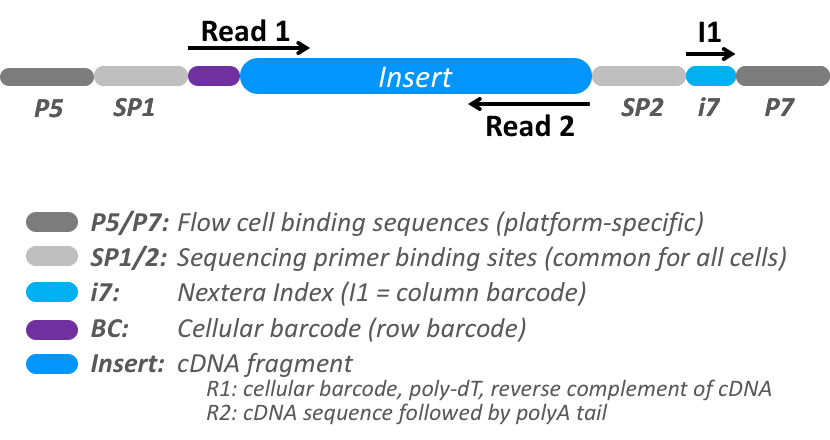
This tutorial will walk you through demultiplexing a fluidigm sequencing run with the PAMLD decoder. The read has 3 segments, 1 biological from the DNA or RNA fragment and 2 technical containing a row cellular barcode in the first 6 cycles of the forward read segment and a column cellular barcode on the first 8 cycles of the i7 index segment.
Input Read Layout
"input": [
    "CBJLFACXX_S1_L001_R1_001.fastq.gz",
    "CBJLFACXX_S1_L001_I1_001.fastq.gz",
    "CBJLFACXX_S1_L001_R2_001.fastq.gz"
]
declaring input read segments Base calling with bc2fastq produced 3 files per lane:
CBJLFACXX_S1_L001_R1_001.fastq.gzcontaining a 6 base pair long row cellular barcode,CBJLFACXX_S1_L001_I1_001.fastq.gzcontaining the 8 base pair column cellular barcode andCBJLFACXX_S1_L001_R2_001.fastq.gzcontaining the reverse complemented 5 prime suffix of the insert region, since it was read in reverse.
In this example our downstream pipeline expected reads for each cell, identified by the combination a row and a column tag, to be in a separate fastq file. Producing so many files makes processing verbose and inefficient, but is sometimes a real world constraint you have to live with to reuse existing code, and demonstrates some of Pheniq’s flexibly. We estimate the prior for the row and column cellular barcodes in a conditional fashion. We will first estimate the prior for the column tag and split the reads matching each column to separate bam file. We then estimate the prior for the row tag independently for each column and further split reads matching each tag to a separate fastq file. We end up with a fastq file for each cell in the table, to match the input for the downstream pipeline.
Column classification
In the first step you classify the reads by the cellular barcode in the i7 segment and split the reads for each column to a separate bam file containing the two remaining segments: the row cellular barcode and the biological sequence. Since the sequences identifying the columns are the same in each lane, you declare a decoder in a CBJLFACXX_core.json that you will reuse in all other configuration files. This decoder lists the possible barcode sequences and a transform that tells Pheniqs where to find the barcode sequence.
Token expression Segment index First Last Length Description 0::60056Row cellular barcode. Used in phase 2 1::81078Column cellular barcode. Used in phase 1 2::20end full cDNA template sequence Tokenization patterns for first phase of classification a fluidigm Row/Column assay. This protocol uses the Nextera XT DNA Library Preparation Kit to apply the row barcodes and the Nextera XT Index Kit v2 to apply the column barcodes. The row barcodes are applied during the reverse transcription (RT) step and are common to all cells in each row. The column barcodes are applied during library preparation to pooled cells from each column and are thus shared by all cells in each column. The complete cellular index for an individual cell is defined by a unique combination of the row (RT) and column (I1) barcodes. The row barcode is in the first 8 bases of Read 1, and the column barcode is in the I1 read. We classify and split the reads by the column barcode and preserve the row column in a segment for decoding in a second phase. The template sequence of biological interest in on the second segment in R2.
{
    "CN": "CGSB AD",
    "PL": "ILLUMINA",
    "PM": "HiSeq",
    "decoder": {
        "@CBJLFACXX_column": {
            "codec": {
                "@AAGAGGCA": {
                    "barcode": [
                        "AAGAGGCA"
                    ]
                },
                "@ACTCGCTA": {
                    "barcode": [
                        "ACTCGCTA"
                    ]
                }
            },
            "transform": {
                "token": [
                    "1::8"
                ]
            }
        }
    },
    "filter incoming qc fail": true,
    "flowcell id": "CBJLFACXX"
}
declaring column demultiplexing The
@CBJLFACXX_columntransform tells Pheniqs where to locate the sequence that should match the column cellular barcode. To discard reads that failed the internal Illumina sequencer chastity filter you instruct Pheniqs to filter incoming QC fail reads with"filter incoming qc fail": true. The actual configuration has more sample barcodes but you only show two here for brevity.
To decode the column cellular barcode for the first lane you create a configuration that will retain the row cellular barcode and the biological sequence in the reverse read.
{
    "flowcell lane number": 1,
    "import": [
        "CBJLFACXX_core.json"
    ],
    "input": [
        "CBJLFACXX_S1_L001_R1_001.fastq.gz",
        "CBJLFACXX_S1_L001_I1_001.fastq.gz",
        "CBJLFACXX_S1_L001_R2_001.fastq.gz"
    ],
    "cellular": {
        "multiplexing classifier": true,
        "algorithm": "pamld",
        "base": "@CBJLFACXX_column",
        "confidence threshold": 0.95,
        "noise": 0.05
    },
    "template": {
        "transform": {
            "token": [
                "0::6",
                "2::"
            ]
        }
    }
}
Classifying reads by the column cellular barcode You keep the cellular tag in a separate segment for further processing in the next phase.
To split the reads by the column cellular barcode into separate bam files you can use the pheniqs-io-api to add the necessary directives to our configuration.
pheniqs-io-api.py \
--split-library \
--format bam \
--configuration CBJLFACXX_l01_column.json \
CBJLFACXX_l01_column_split.json
This will create the CBJLFACXX_l01_column_split.json with additional output directives for each barcode.
{
    "flowcell lane number": 1,
    "import": [
        "CBJLFACXX_core.json"
    ],
    "input": [
        "CBJLFACXX_S1_L001_R1_001.fastq.gz",
        "CBJLFACXX_S1_L001_I1_001.fastq.gz",
        "CBJLFACXX_S1_L001_R2_001.fastq.gz"
    ],
    "cellular": {
        "multiplexing classifier": true,
        "algorithm": "pamld",
        "base": "@CBJLFACXX_column",
        "codec": {
            "@AAGAGGCA": {
                "output": [
                    "CBJLFACXX_AAGAGGCA.bam"
                ]
            },
            "@ACTCGCTA": {
                "output": [
                    "CBJLFACXX_ACTCGCTA.bam"
                ]
            }
        },
        "confidence threshold": 0.95,
        "noise": 0.05,
        "undetermined": {
            "output": [
                "CBJLFACXX_undetermined.bam"
            ]
        }
    },
    "template": {
        "transform": {
            "token": [
                "0::6",
                "2::"
            ]
        }
    }
}
splitting by the column cellular barcode with the
pheniqs-io-apiadds anoutputdirective to each barcode in the codec. File names use theLBauxiliary tag, if available, or the barcode sequence otherwise.
You can validate the configuration with Pheniqs. The validation output is a readable description of all the explicit and implicit parameters after applying defaults. You can check how Pheniqs detects the input format, compression and layout as well as the output you can expect. In The Output transform section you can find a verbal description of how the output read segments will be assembled from the input. similarly Transform in the Mutliplex decoding section describes how the segment that will be matched against the barcodes is assembled. You can also see how each of the read groups will be tagged and the prior probability PAMLD will assume for each barcode. Since no prior was provided, Pheniqs computes the uniform prior.
pheniqs mux --config CBJLFACXX_l01_column.json --validate
We can also examine the compile configuration, which is the actual configuration Pheniqs will execute with all implicit and default parameters. This is an easy way to see exactly what Pheniqs will be doing and spotting any configuration errors.
pheniqs mux --config CBJLFACXX_l01_column.json --compile
Prior estimation
Better estimation of the prior distribution improves accuracy. The pheniqs-prior-api can adjust your configuration to include priors estimated from a report emitted by a preliminary run. The priors you specify in your initial configuration can be your best guess for the priors but you can simply leave them out altogether, which assumes a uniform prior. Since you are only interested in collecting statistics and not the output from this run, you create an optimized configuration that will execute much faster by only examining the relevant input and produce no sequence output. CBJLFACXX_l01_column_estimate.json declares a cellular directive that expands CBJLFACXX_column and adjusts the tokenization for the modified input. output is redirected to /dev/null to tell Pheniqs it should not bother with the output.
{
    "flowcell lane number": 1,
    "import": [
        "CBJLFACXX_core.json"
    ],
    "input": [
        "CBJLFACXX_S1_L001_I1_001.fastq.gz"
    ],
    "cellular": {
        "multiplexing classifier": true,
        "algorithm": "pamld",
        "base": "@CBJLFACXX_column",
        "confidence threshold": 0.95,
        "noise": 0.05,
        "transform": {
            "token": [
                "0::8"
            ]
        }
    },
    "output": [
        "/dev/null"
    ],
    "report url": "CBJLFACXX_l01_column_estimate_report.json",
    "template": {
        "transform": {
            "token": [
                "0::8"
            ]
        }
    }
}
Column Prior estimation configuration refrains from reading the biological sequences and produces no output which significantly speeds things up.
Executing CBJLFACXX_l01_column_estimate.json will yield the CBJLFACXX_l01_column_estimate_report.json report. Like every Pheniqs report, it contains decoding statistics that you can use to estimate the priors.
pheniqs mux --config CBJLFACXX_l01_column_estimate.json
Now that you have CBJLFACXX_l01_column_split.json, a decoding configuration, and CBJLFACXX_l01_column_estimate_report.json, a report with decoding statistics, you can use pheniqs-prior-api to generate a prior adjusted configuration file.
pheniqs-prior-api.py \
--report CBJLFACXX_l01_column_estimate_report.json \
--configuration CBJLFACXX_l01_column_split.json \
CBJLFACXX_l01_column_adjusted.json
column barcode decoding with an estimated prior CBJLFACXX_l01_column_adjusted.json is similar to CBJLFACXX_l01_column_split.json with the addition of the estimated priors.
This will produce CBJLFACXX_l01_sample_estimated.json, a new configuration file with the adjusted priors. The method for estimating the prior is described in the manual and makes some assumptions about the preparation protocol. You can also devise your own methods of estimating the priors and plug them into the configuration.
You can now proceed to demultiplex the column cellular barcode with the adjusted configuration and produce a separate bam file with reads from each column.
pheniqs mux --config CBJLFACXX_l01_column_adjusted.json
Row classification
In the first step you produced multiple bam files, one for each column. In this second phase you will estimate priors and decode the row cellular barcode on each of those bam files independently. Notice that this time you only have 2 input segments. The first is the 6 base pair row cellular barcode and the second is the DNA or RNA fragment. Since you want to reuse configuration files in this step for every one of the bam files you produced in the first step you intentionally leave out the input and output directive and will specify them on the command line.
Token expression Segment index First Last Length Description 0::60056Row cellular barcode. 1::10end full cDNA template sequence Tokenization patterns for second phase, splitting a single column into cells by the row barcode. The first phase produced 2 segments: first with the 6 nucleotides of the row barcode and the second with the cDNA template sequence. In this second phase we classify by the row barcode and discard it, emitting the cDNA template sequence.
First we write the configuration file for decoding the row tag
{
    "flowcell lane number": 1,
    "import": [
        "CBJLFACXX_core.json"
    ],
    "cellular": {
        "multiplexing classifier": true,
        "algorithm": "pamld",
        "base": "@CBJLFACXX_row",
        "confidence threshold": 0.95,
        "noise": 0.05,
        "transform": {
            "token": [
                "0::6"
            ]
        }
    },
    "template": {
        "transform": {
            "token": [
                "1::"
            ]
        }
    }
}
Classifying by the row cellular barcode using the bam files produced in the first step.
To estimate the row cellular barcode prior we have a similar reusable configuration
{
    "flowcell lane number": 1,
    "import": [
        "CBJLFACXX_core.json"
    ],
    "cellular": {
        "multiplexing classifier": true,
        "algorithm": "pamld",
        "base": "@CBJLFACXX_row",
        "confidence threshold": 0.95,
        "noise": 0.05,
        "transform": {
            "token": [
                "0::6"
            ]
        }
    },
    "output": [
        "/dev/null"
    ],
    "template": {
        "transform": {
            "token": [
                "0::6"
            ]
        }
    }
}
Row prior estimation configuration** will produce statistics about the bam files produced in the first step.
We can execute the prior estimation configuration on each column bam file using a simple shell loop
for file in *.bam; do
pheniqs mux --config CBJLFACXX_l01_row_estimate.json --input "$file" --report "${x/.bam/_estimate_report.json}";
done;
estimating cellular priors this shell loop will execute Pheniqs for each of the bam files produced in the first phase.
To create a splitting configuration for each column bam file we use the pheniqs-io-api again
for file in *.bam; do
pheniqs-io-api.py \
--split-library \
--format fastq \
--configuration CBJLFACXX_l01_row.json \
--input "$file" \
--input "$file" \
--prefix "${file/.bam/}" \
"${file/.bam/_split.json}"
done;
generating a splitting configuration for each column by row this will produce a splitting configuration for each of the bam files produced in the first phase.
adjusting the priors on each with pheniqs-prior-api
for file in *.bam; do
pheniqs-prior-api.py \
--report "${x/.bam/_estimate_report.json}" \
--configuration "${file/.bam/_split.json}" \
"${file/.bam/_adjusted.json}"
estimating row priors on each column this will produce a splitting configuration for each of the bam files produced in the first phase.
and finally executing the adjusted configuration
for file in *.bam; do
pheniqs mux \
--config "${file/.bam/_adjusted.json}" \
--report "${x/.bam/_report.json}"
splitting each column by row this will produce a splitting configuration for each of the bam files produced in the first phase.